10 - Matching#

What is Regression Doing After All?#

As we’ve seen so far, regression does an amazing job at controlling for additional variables when we do a test vs control comparison. If we have independence, \((Y_0, Y_1)\perp T | X\), then regression can identify the ATE by controlling for X. The way regression does this is kind of magical. To get some intuition about it, let’s remember the case when all variables X are dummy variables. If that is the case, regression partitions the data into the dummy cells and computes the mean difference between test and control. This difference in means keeps the Xs constant, since we are doing it in a fixed cell of X dummy. It is as if we were doing \(E[Y|T=1] - E[Y|T=0] | X=x\), where \(x\) is a dummy cell (all dummies set to 1, for example). Regression then combines the estimate in each of the cells to produce a final ATE. The way it does this is by applying weights to the cell proportional to the variance of the treatment on that group.

import warnings
warnings.filterwarnings('ignore')

import pandas as pd
import numpy as np
from matplotlib import style
from matplotlib import pyplot as plt
import statsmodels.formula.api as smf

import graphviz as gr

%matplotlib inline

style.use("fivethirtyeight")

To give an example, let’s suppose I’m trying to estimate the effect of a drug and I have 6 men and 4 women. My response variable is days hospitalised and I hope my drug can lower that. On men, the true causal effect is -3, so the drug lowers the stay period by 3 days. On women, it is -2. To make matters more interesting, men are much more affected by this illness and stay longer at the hospital. They also get much more of the drug. Only 1 out of the 6 men does not get the drug. On the other hand, women are more resistant to this illness, so they stay less at the hospital. 50% of the women get the drug.

drug_example = pd.DataFrame(dict(
    sex= ["M","M","M","M","M","M", "W","W","W","W"],
    drug=[1,1,1,1,1,0,  1,0,1,0],
    days=[5,5,5,5,5,8,  2,4,2,4]
))

Note that simple comparison of treatment and control yields a negatively biased effect, that is, the drug seems less effective than it truly is. This is expected, since we’ve omitted the sex confounder. In this case, the estimated ATE is smaller than the true one because men get more of the drug and are more affected by the illness.

drug_example.query("drug==1")["days"].mean() - drug_example.query("drug==0")["days"].mean()

-1.1904761904761898

Since the true effect for men is -3 and the true effect for women is -2, the ATE should be

\( ATE=\dfrac{(-3*6) + (-2*4)}{10}=-2.6 \)

This estimate is done by 1) partitioning the data into confounder cells, in this case, men and women, 2) estimating the effect on each cell and 3) combining the estimate with a weighted average, where the weight is the sample size of the cell or covariate group. If we had exactly the same number of men and women in the data, the ATE estimate would be right in the middle of the ATE of the 2 groups, -2.5. Since there are more men than women in our dataset, the ATE estimate is a little bit closer to the men’s ATE. This is called a non-parametric estimate, since it places no assumption on how the data was generated.

If we control for sex using regression, we will add the assumption of linearity. Regression will also partition the data into men and women and estimate the effect on both of these groups. So far, so good. However, when it comes to combining the effect on each group, it does not weigh them by the sample size. Instead, regression uses weights that are proportional to the variance of the treatment in that group. In our case, the variance of the treatment in men is smaller than in women, since only one man is in the control group. To be exact, the variance of T for men is \(0.139=1/6*(1 - 1/6)\) and for women is \(0.25=2/4*(1 - 2/4)\). So regression will give a higher weight to women in our example and the ATE will be a bit closer to the women’s ATE of -2.

smf.ols('days ~ drug + C(sex)', data=drug_example).fit().summary().tables[1]

	coef	std err	t	P>\|t\|	[0.025	0.975]
Intercept	7.5455	0.188	40.093	0.000	7.100	7.990
C(sex)[T.W]	-3.3182	0.176	-18.849	0.000	-3.734	-2.902
drug	-2.4545	0.188	-13.042	0.000	-2.900	-2.010

This result is more intuitive with dummy variables, but, in its own weird way, regression also keeps continuous variables constant while estimating the effect. Also with continuous variables, the ATE will point in the direction where covariates have more variance.

So we’ve seen that regression has its idiosyncrasies. It is linear, parametric, likes high variance features… This can be good or bad, depending on the context. Because of this, it’s important to be aware of other techniques we can use to control for confounders. Not only are they an extra tool in your causal tool belt, but understanding different ways to deal with confounding expands our understanding of the problem. For this reason, I present you now the Subclassification Estimator!

The Subclassification Estimator#

If there is some causal effect we want to estimate, like the effect of job training on earnings, and the treatment is not randomly assigned, we need to watch out for confounders. It could be that only more motivated people do the training and they would have higher earnings regardless of the training. We need to estimate the effect of the training program within small groups of individuals that are roughly the same in motivation level and any other confounders we may have.

More generally, if there is some causal effect we want to estimate, but it is hard to do so because of confounding of some variables X, what we need to do is make the treatment vs control comparison within small groups where X is the same. If we have conditional independence \((Y_0, Y_1)\perp T | X\), then we can write the ATE as follows.

\( ATE = \int(E[Y|X, T=1] - E[Y|X, T=0])dP(x) \)

What this integral does is it goes through all the space of the distribution of features X, computes the difference in means for all those tiny spaces and combines everything into the ATE. Another way to see this is to think about a discrete set of features. In this case, we can say that the features X takes on K different cells \(\{X_1, X_2, ..., X_k\}\) and what we are doing is computing the treatment effect in each cell and combining them into the ATE. In this discrete case, converting the integral to a sum, we can derive the subclassifications estimator

\( \hat{ATE} = \sum^K_{k=1}(\bar{Y}_{k1} - \bar{Y}_{k0}) * \dfrac{N_k}{N} \)

where the bar represent the mean of the outcome on the treated, \(Y_{k1}\), and non-treated, \(Y_{k0}\), at cell k and \(N_{k}\) is the number of observations in that same cell. As you can see, we are computing a local ATE for each cell and combining them using a weighted average, where the weights are the sample size of the cell. In our medicine example above, this would be the first estimate, which gave us −2.6.

Matching Estimator#

The subclassification estimator isn’t used much in practice (we will see why shortly, it is because of the curse of dimensionality) but it gives us a nice intuition of what a causal inference estimator should do, how it should control for confounders. This allows us to explore other kinds of estimators, such as the Matching Estimator.

The idea is very similar. Since some sort of confounder X makes it so that treated and untreated are not initially comparable, I can make them so by matching each treated unit with a similar untreated unit. It is like I’m finding an untreated twin for every treated unit. By making such comparisons, treated and untreated become again comparable.

As an example, let’s suppose we are trying to estimate the effect of a trainee program on earnings. Here is what the trainees looks like

trainee = pd.read_csv("./data/trainees.csv")
trainee.query("trainees==1")

	unit	trainees	age	earnings
0	1	1	28	17700
1	2	1	34	10200
2	3	1	29	14400
3	4	1	25	20800
4	5	1	29	6100
5	6	1	23	28600
6	7	1	33	21900
7	8	1	27	28800
8	9	1	31	20300
9	10	1	26	28100
10	11	1	25	9400
11	12	1	27	14300
12	13	1	29	12500
13	14	1	24	19700
14	15	1	25	10100
15	16	1	43	10700
16	17	1	28	11500
17	18	1	27	10700
18	19	1	28	16300

And here are the non-trainees:

trainee.query("trainees==0")

	unit	age	earnings
19	20	43	20900
20	21	50	31000
21	22	30	21000
22	23	27	9300
23	24	54	41100
24	25	48	29800
25	26	39	42000
26	27	28	8800
27	28	24	25500
28	29	33	15500
29	31	26	400
30	32	31	26600
31	33	26	16500
32	34	34	24200
33	35	25	23300
34	36	24	9700
35	37	29	6200
36	38	35	30200
37	39	32	17800
38	40	23	9500
39	41	32	25900

If I do a simple comparison in means, we get that the trainees earn less money than those that didn’t go through the program.

trainee.query("trainees==1")["earnings"].mean() - trainee.query("trainees==0")["earnings"].mean()

-4297.49373433584

However, if we look at the table above, we notice that trainees are much younger than non trainees, which indicates that age is probably a confounder. Let’s use matching on age to try to correct that. We will take unit 1 from the treated and pair it with unit 27, since both are 28 years old. Unit 2 we will pair it with unit 34, unit 3 with unit 37, unit 4 we will pair it with unit 35… When it comes to unit 5, we need to find someone with age 29 from the non treated, but that is unit 37, which is already paired. This is not a problem, since we can use the same unit multiple times. If more than 1 unit is a match, we can choose randomly between them.

This is what the matched dataset looks like for the first 7 units

# make dataset where no one has the same age
unique_on_age = (trainee
                 .query("trainees==0")
                 .drop_duplicates("age"))

matches = (trainee
           .query("trainees==1")
           .merge(unique_on_age, on="age", how="left", suffixes=("_t_1", "_t_0"))
           .assign(t1_minuts_t0 = lambda d: d["earnings_t_1"] - d["earnings_t_0"]))

matches.head(7)

	unit_t_1	trainees_t_1	age	earnings_t_1	unit_t_0	earnings_t_0	t1_minuts_t0
0	1	1	28	17700	27	8800	8900
1	2	1	34	10200	34	24200	-14000
2	3	1	29	14400	37	6200	8200
3	4	1	25	20800	35	23300	-2500
4	5	1	29	6100	37	6200	-100
5	6	1	23	28600	40	9500	19100
6	7	1	33	21900	29	15500	6400

Notice how the last column has the difference in earnings between the treated and its matched untreated unit. If we take the mean of this last column we get the ATET estimate while controlling for age. Notice how the estimate is now very positive, compared to the previous one where we used a simple difference in means.

matches["t1_minuts_t0"].mean()

2457.8947368421054

But this was a very contrived example, just to introduce matching. In reality, we usually have more than one feature and units don’t match perfectly. In this case, we have to define some measurement of proximity to compare how units are close to each other. One common metric for this is the euclidean norm \(||X_i - X_j||\). This difference, however, is not invariant to the scale of the features. This means that features like age, that take values on the tenths, will be much less important when computing this norm compared to features like income, which take the order of hundreds. For this reason, before applying the norm, we need to scale the features so that they are on roughly the same scale.

Having defined a distance measure, we can now define the match as the nearest neighbour to that sample we wish to match. In math terms, we can write the matching estimator the following way

\( \hat{ATE} = \frac{1}{N} \sum^N_{i=1} (2T_i - 1)\big(Y_i - Y_{jm}(i)\big) \)

Where \(Y_{jm}(i)\) is the sample from the other treatment group which is most similar to \(Y_i\). We do this \(2T_i - 1\) to match both ways: treated with controls and controls with the treatment.

To test this estimator, let’s consider a medicine example. Once again, we want to find the effect of a medication on days until recovery. Unfortunately, this effect is confounded by severity, sex and age. We have reasons to believe that patients with more severe conditions have a higher chance of receiving the medicine.

med = pd.read_csv("./data/medicine_impact_recovery.csv")
med.head()

	sex	age	severity	medication	recovery
0	0	35.049134	0.887658	1	31
1	1	41.580323	0.899784	1	49
2	1	28.127491	0.486349	0	38
3	1	36.375033	0.323091	0	35
4	0	25.091717	0.209006	0	15

If we look at a simple difference in means, \(E[Y|T=1]-E[Y|T=0]\), we get that the treatment takes, on average, 16.9 more days to recover than the untreated. This is probably due to confounding, since we don’t expect the medicine to cause harm to the patient.

med.query("medication==1")["recovery"].mean() - med.query("medication==0")["recovery"].mean()

16.895799546498726

To correct for this bias, we will control for X using matching. First, we need to remember to scale our features, otherwise, features like age will have higher importance than features like severity when we compute the distance between points. To do so, we can standardise the features.

# scale features
X = ["severity", "age", "sex"]
y = "recovery"

med = med.assign(**{f: (med[f] - med[f].mean())/med[f].std() for f in X})
med.head()

	sex	age	severity	medication	recovery
0	-0.996980	0.280787	1.459800	1	31
1	1.002979	0.865375	1.502164	1	49
2	1.002979	-0.338749	0.057796	0	38
3	1.002979	0.399465	-0.512557	0	35
4	-0.996980	-0.610473	-0.911125	0	15

Now, to the matching itself. Instead of coding a matching function, we will use the K nearest neighbour algorithm from Sklearn. This algorithm makes predictions by finding the nearest data point in an estimation or training set.

For matching, we will need 2 of those. One, mt0, will store the untreated points and will find matches in the untreated when asked to do so. The other, mt1, will store the treated point and will find matches in the treated when asked to do so. After this fitting step, we can use these KNN models to make predictions, which will be our matches.

from sklearn.neighbors import KNeighborsRegressor

treated = med.query("medication==1")
untreated = med.query("medication==0")

mt0 = KNeighborsRegressor(n_neighbors=1).fit(untreated[X], untreated[y])
mt1 = KNeighborsRegressor(n_neighbors=1).fit(treated[X], treated[y])

predicted = pd.concat([
    # find matches for the treated looking at the untreated knn model
    treated.assign(match=mt0.predict(treated[X])),
    
    # find matches for the untreated looking at the treated knn model
    untreated.assign(match=mt1.predict(untreated[X]))
])

predicted.head()

	sex	age	severity	medication	recovery	match
0	-0.996980	0.280787	1.459800	1	31	39.0
1	1.002979	0.865375	1.502164	1	49	52.0
7	-0.996980	1.495134	1.268540	1	38	46.0
10	1.002979	-0.106534	0.545911	1	34	45.0
16	-0.996980	0.043034	1.428732	1	30	39.0

With the matches, we can now apply the matching estimator formula

\( \hat{ATE} = \frac{1}{N} \sum^N_{i=1} (2T_i - 1)\big(Y_i - Y_{jm}(i)\big) \)

np.mean((2*predicted["medication"] - 1)*(predicted["recovery"] - predicted["match"]))

-0.9954

Using this sort of matching, we can see that the effect of the medicine is not positive anymore. This means that, controlling for X, the medicine reduces the recovery time by about 1 day, on average. This is already a huge improvement on top of the biased estimate that predicted a 16.9 increase in recovery time.

However, we can still do better.

Matching Bias#

It turns out the matching estimator as we’ve designed above is biased. To see this, let’s consider the ATET estimator, instead of the ATE, just because it is simpler to write. The intuition will apply to the ATE as well.

\( \hat{ATET} = \frac{1}{N_1}\sum (Y_i - Y_j(i)) \)

where \(N_1\) is the number of treated individuals and \(Y_j(i)\) is the untreated match of treated unit i. To check for bias, what we do is hope we can apply the Central Limit Theorem so that this down there converges to a normal distribution with mean zero.

\( \sqrt{N_1}(\hat{ATET} - ATET) \)

However, this doesn’t alway happen. If we define the mean outcome for the untreated given X, \(\mu_0(x)=E[Y|X=x, T=0]\), we will have that (btw, I’ve omitted the proof for that because it’s a little beyond the point here).

\( E[\sqrt{N_1}(\hat{ATET} - ATET)] = E[\sqrt{N_1}(\mu_0(X_i) - \mu_0(X_j(i)))] \)

Now, \(\mu_0(X_i) - \mu_0(X_j(i))\) is not so simple to understand, so let’s look at it more carefully. \(\mu_0(X_i)\) is the outcome Y value of a treated unit \(i\) had it not been treated. So, it is the counterfactual outcome \(Y_0\) for unit i. \(\mu_0(X_j(i))\) is the outcome of the untreated unit \(j\) that is the match of unit \(i\). So, it is also the \(Y_0\) , but for unit \(j\) now. Only this time, it is a factual outcome, because \(j\) is in the non treated group. Now, because \(j\) and \(i\) are only similar, but not the same, this will likely not be zero. In other words, \(X_i \approx X_j \). So, \(Y_{0i} \approx Y_{0j} \).

As we increase the sample size, there will be more units to match, so the difference between unit \(i\) and its match \(j\) will also get smaller. But this difference converges to zero slowly. As a result \(E[\sqrt{N_1}(\mu_0(X_i) - \mu_0(X_j(i)))]\) may not converge to zero, because the \(\sqrt{N_1}\) grows faster than \((\mu_0(X_i) - \mu_0(X_j(i)))\) diminishes.

Bias arises when the matching discrepancies are huge. Fortunately, we know how to correct it. Each observation contributes \((\mu_0(X_i) - \mu_0(X_j(i)))\) to the bias so all we need to do is subtract this quantity from each matching comparison in our estimator. To do so, we can replace \(\mu_0(X_j(i))\) with some sort of estimate of this quantity \(\hat{\mu_0}(X_j(i))\), which can be obtained with models like linear regression. This updates the ATET estimator to the following equation

\( \hat{ATET} = \frac{1}{N_1}\sum \big((Y_i - Y_{j(i)}) - (\hat{\mu_0}(X_i) - \hat{\mu_0}(X_{j(i)}))\big) \)

where \(\hat{\mu_0}(x)\) is some estimative of \(E[Y|X, T=0]\), like a linear regression fitted only on the untreated sample.

from sklearn.linear_model import LinearRegression

# fit the linear regression model to estimate mu_0(x)
ols0 = LinearRegression().fit(untreated[X], untreated[y])
ols1 = LinearRegression().fit(treated[X], treated[y])

# find the units that match to the treated
treated_match_index = mt0.kneighbors(treated[X], n_neighbors=1)[1].ravel()

# find the units that match to the untreatd
untreated_match_index = mt1.kneighbors(untreated[X], n_neighbors=1)[1].ravel()

predicted = pd.concat([
    (treated
     # find the Y match on the other group
     .assign(match=mt0.predict(treated[X])) 
     
     # build the bias correction term
     .assign(bias_correct=ols0.predict(treated[X]) - ols0.predict(untreated.iloc[treated_match_index][X]))),
    (untreated
     .assign(match=mt1.predict(untreated[X]))
     .assign(bias_correct=ols1.predict(untreated[X]) - ols1.predict(treated.iloc[untreated_match_index][X])))
])

predicted.head()

	sex	age	severity	medication	recovery	match	bias_correct
0	-0.996980	0.280787	1.459800	1	31	39.0	4.404034
1	1.002979	0.865375	1.502164	1	49	52.0	12.915348
7	-0.996980	1.495134	1.268540	1	38	46.0	1.871428
10	1.002979	-0.106534	0.545911	1	34	45.0	-0.496970
16	-0.996980	0.043034	1.428732	1	30	39.0	2.610159

One immediate question that arises is: doesn’t this defeat the point of matching? If I have to run a linear regression anyway, why don’t I use only that, instead of this complicated model. That’s a fair point, so I should take some time to answer it.

First of all, this linear regression that we are fitting doesn’t extrapolate on the treatment dimension to get the treatment effect. Instead, its purpose is just to correct bias. Linear regression here is local, in the sense that it doesn’t try to see how the treated would be if it looked like the untreated. It does none of that extrapolation. This is left to the matching part. The meat of the estimator is still the matching component. The point I want to make here is that OLS is secondary to this estimator.

The second point is that matching is a non-parametric estimator. It doesn’t assume linearity or any kind of parametric model. As such, it is more flexible than linear regression and can work in situations where linear regression will not, namely, those where non linearity is very strong.

Does this mean that you should only use matching? Well, that’s a tough question. Alberto Abadie makes a case that yes, you should. It’s more flexible and, once you have the code, equally simple to run. I’m not entirely convinced by that. For example, Abadie spent a lot of time studying and developing the estimator (yes, he is one of the scientists that contributes to matching being what it is), so he obviously is personally invested in the method. Second, there is something about linear regression’s simplicity that you don’t see in matching. The partial derivative math of “holding everything else constant” is much easier to grasp with linear regression than with matching. But that’s just my preference. To be honest, there is no clear answer to this question. Anyway, back to our example.

With the bias correction formula, I get the following ATE estimation.

np.mean((2*predicted["medication"] - 1)*((predicted["recovery"] - predicted["match"])-predicted["bias_correct"]))

-7.36266090614141

Of course, we also need to place a confidence interval around this measurement, but enough of math theory now. In practice, we can simply use someone else’s code and just import a matching estimator. Here is one from the library causalinference.

from causalinference import CausalModel

cm = CausalModel(
    Y=med["recovery"].values, 
    D=med["medication"].values, 
    X=med[["severity", "age", "sex"]].values
)

cm.est_via_matching(matches=1, bias_adj=True)

print(cm.estimates)

Treatment Effect Estimates: Matching

                     Est.       S.e.          z      P>|z|      [95% Conf. int.]
--------------------------------------------------------------------------------
           ATE     -7.709      0.609    -12.649      0.000     -8.903     -6.514
           ATC     -6.665      0.246    -27.047      0.000     -7.148     -6.182
           ATT     -9.679      1.693     -5.717      0.000    -12.997     -6.361

Finally, we can say with confidence that our medicine does indeed lower the time someone spends at the hospital. The ATE estimate is just a little bit lower than mine, due to the difference in tie breaking of matches of knn sklearn implementation and the causalinference python package.

Before we close this topic, I just wanted to address the cause of bias in matching a little bit more. We saw that matching is biased when the unit and its match are not so similar. But what causes them to be so different?

The Curse of Dimensionality#

As it turns out, the answer is quite simple and intuitive. It is easy to find people that match on a few characteristics, like sex. But if we add more characteristics, like age, income, city of birth and so on, it becomes harder and harder to find matches. In more general terms, the more features we have, the higher will be the distance between units and their matches.

This is not something that hurts only the matching estimator. It ties back to the subclassification estimator we saw earlier. Early on, in that contrived medicine example where with man and woman, it was quite easy to build the subclassification estimator. That was because we only had 2 cells: man and woman. But what would happen if we had more? Let’s say we have 2 continuous features like age and income and we manage to discretise them into 5 buckets each. This will give us 25 cells, or \(5^2\). And what if we had 10 covariates with 3 buckets each? Doesn’t seem like a lot right? Well, this would give us 59049 cells, or \(3^{10}\). It’s easy to see how this can blow out of proportion pretty quickly. This is a phenomena pervasive in all data science, which is called the The Curse of Dimensionality!!!

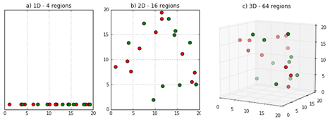
Image Source: https://deepai.org/machine-learning-glossary-and-terms/curse-of-dimensionality

Despite its scary and pretentious name, this only means that the number of data points required to fill a feature space grows exponentially with the number of features, or dimensions. So, if it takes X data points to fill the space of, say, 3 feature spaces, it takes exponentially more points to fill in the space of 4 features.

In the context of the subclassification estimator, the curse of dimensionality means that it will suffer if we have lots of features. Lots of features imply multiple cells in X. If there are multiple cells, some of them will have very few data. Some of them might even have only treated or only control, so it won’t be possible to estimate the ATE there, which would break our estimator. In the matching context, this means that the feature space will be very sparse and units will be very far from each other. This will increase the distance between matches and cause bias problems.

As for linear regression, it actually handles this problem quite well. What it does is project all the features X into a single one, the Y dimension. It then makes treatment and control comparison on that projection. So, in some way, linear regression performs some sort of dimensionality reduction to estimate the ATE. It’s quite elegant.

Most causal models also have some way to deal with the curse of dimensionality. I won’t keep repeating myself, but it is something you should keep in mind when looking at them. For instance, when we deal with propensity scores in the following section, try to see how it solves this problem.

Key Ideas#

We’ve started this section understanding what linear regression does and how it can help us identify causal relationships. Namely, we understood that regression can be seen as partitioning the dataset into cells, computing the ATE in each cell and then combining the cell’s ATE into a single ATE for the entire dataset.

From there, we’ve derived a very general causal inference estimator with subclassification. We saw how that estimator is not very useful in practice but it gave us some interesting insights on how to tackle the problem of causal inference estimation. That gave us the opportunity to talk about the matching estimator.

Matching controls for the confounders by looking at each treated unit and finding an untreated pair that is very similar to it and similarly for the untreated units. We saw how to implement this method using the KNN algorithm and also how to debiase it using regression. Finally, we discussed the difference between matching and linear regression. We saw how matching is a non parametric estimator that doesn’t rely on linearity the way linear regression does.

Finally, we’ve delved into the problem of high dimensional datasets and we saw how causal inference methods can suffer from it.

References#

I like to think of this entire book as a tribute to Joshua Angrist, Alberto Abadie and Christopher Walters for their amazing Econometrics class. Most of the ideas here are taken from their classes at the American Economic Association. Watching them is what is keeping me sane during this tough year of 2020.

I’ll also like to reference the amazing books from Angrist. They have shown me that Econometrics, or ‘Metrics as they call it, is not only extremely useful but also profoundly fun.

My final reference is Miguel Hernan and Jamie Robins’ book. It has been my trustworthy companion in the most thorny causal questions I had to answer.

Causal Inference Book

Contribute#

Causal Inference for the Brave and True is an open-source material on causal inference, the statistics of science. It uses only free software, based in Python. Its goal is to be accessible monetarily and intellectually. If you found this book valuable and you want to support it, please go to Patreon. If you are not ready to contribute financially, you can also help by fixing typos, suggesting edits or giving feedback on passages you didn’t understand. Just go to the book’s repository and open an issue. Finally, if you liked this content, please share it with others who might find it useful and give it a star on GitHub.

Causal Inference for the Brave and True

10 - Matching

Contents