14 - Panel Data and Fixed Effects#
In the previous chapter, we explored a very simple Diff-in-Diff setup, where we had a treated and a control group (the city of POA and FLN, respectively) and only two periods, a pre-intervention and a post-intervention period. But what would happen if we had more periods? Or more groups? Turns out this setup is so common and powerful for causal inference that it gets its own name: panel data. A panel is when we have repeated observations of the same unit over multiple periods of time. This happens a lot in government policy evaluation, where we can track data on multiple cities or states over multiple years. But it is also incredibly common in the industry, where companies track user data over multiple weeks and months.
To understand how we can leverage such data structure, let’s first continue with our diff-in-diff example, where we wanted to estimate the impact of placing a billboard (treatment) in the city of Porto Alegre (POA). We want to see if that sort of offline marketing strategy can boost the usage of our investment products. Specifically, we want to know how much deposits in our investments account would increase if we placed billboards.
In the previous chapter, we’ve motivated the DiD estimator as an imputation strategy of what would have happened to Porto Alegre had we not placed the billboards in it. We said that the counterfactual outcome \(Y_0\) for Porto Alegre after the intervention (placing a billboard) could be inputted as the number of deposits in Porto Alegre before the intervention plus a growth factor. This growth factor was estimated in a control city, Florianopolis (FLN). Just so we can recap some notation, here is how we can estimate this counterfactual outcome
where \(t\) denotes time, \(D\) denotes the treatment (since \(t\) is taken), \(Y_D(t)\) denote the potential outcome for treatment \(D\) in period \(t\) (for example, \(Y_0(1)\) is the outcome under the control in period 1). Now, if we take that imputed potential outcome, we can recover the treatment effect for POA (ATT) as follows
In other words, the effect of placing a billboard in POA is the outcome we saw on POA after placing the billboard minus our estimate of what would have happened if we hadn’t placed the billboard. Also, recall that the power of DiD comes from the fact that estimating the mentioned counterfactual only requires that the growth deposits in POA matches the growth in deposits in FLN. This is the key parallel trends assumption. We should definitely spend some time on it because it is going to become very important later on.
Parallel Trends#
One way to see the parallel (or common) trends assumptions is as an independence assumption. If we recall from very early chapters, the independence assumption requires that the treatment assignment is independent from the potential outcomes:
This means we don’t give more treatment to units with higher outcome (which would cause upward bias in the effect estimation) or lower outcome (which would cause downward bias). In less abstract terms, back to our example, let’s say that your marketing manager decides to add billboards only to cities that already have very high deposits. That way, he or she can later boast that cities with billboards generate more deposites, so of course the marketing campaign was a success. Setting aside the moral discussion here, I think you can see that this violates the independence assumption: we are giving the treatment to cities with high \(Y_0\). Also, remember that a natural extension of this assumption is the conditional independence assumption, which allows the potential outcomes to be dependent on the treatment at first, but independent once we condition on the confounders \(X\)
\( Y_d \perp D | X \)
You know all of this already. But how exactly does this tie back to DiD and the parallel trends assumption? If the traditional independence assumption states that the treatment assignment can’t be related to the levels of potential outcomes, the parallel trends states that the treatment assignment can’t be related to the growth in potential outcomes over time. In fact, one way to write the parallel trends assumption is as follows
\( \big(Y_d(t) - Y_d(t-1) \big) \perp D \)
In less mathematical terms, this assumption is saying it is fine that we assign the treatment to units that have a higher or lower level of the outcome. What we can’t do is assign the treatment to units based on how the outcome is growing. In our billboard example, this means it is OK to place billboards only in cities with originally high deposits level. What we can’t do is place billboards only in cities where the deposits are growing the most. That makes a lot of sense if we remember that DiD is inputting the counterfactual growth in the treated unit with the growth in the control unit. If growth in the treated unit under the control is different than the growth in the control unit, then we are in trouble.
Controlling What you Cannot See#
Methods like propensity score, linear regression and matching are very good at controlling for confounding in non-random data, but they rely on a key assumption: conditional unconfoundedness
\( (Y_0, Y_1) \perp T | X \)
To put it in words, they require that all the confounders are known and measured, so that we can condition on them and make the treatment as good as random. One major issue with this is that sometimes we simply can’t measure a confounder. For instance, take a classical labor economics problem of figuring out the impact of marriage on men’s earnings. It’s a well known fact in economics that married men earn more than single men. However, it is not clear if this relationship is causal or not. It could be that more educated men are both more likely to marry and more likely to have a high earnings job, which would mean that education is a confounder of the effect of marriage on earnings. For this confounder, we could measure the education of the person in the study and run a regression controlling for that. But another confounder could be beauty. It could be that more handsome men are both more likely to get married and more likely to have a high paying job. Unfortunately, beauty is one of those characteristics like intelligence. It’s something we can’t measure very well.
This puts us in a difficult situation, because if we have unmeasured confounders, we have bias. One way to deal with this is with instrumental variables, as we’ve seen before. But coming up with good instruments it’s no easy task and requires a lot of creativity. Here, instead let’s take advantage of our panel data structure.
We’ve already seen how panel data allows us to replace the unconfoundedness assumption with the parallel trends assumption. But how exactly does this help with unmeasured confounders? First, let’s take a look at the causal graph which represents this setup where we have repeated observations across time. Here, we track the same observation across 4 time periods. Marriage (the treatment) and Income (the outcome) change over time. Specifically, marriage turns on (from 0 to 1) at period 3 and 4 and income increases in the same periods. Beauty, the unmeasured confounder, is the same across all periods (a bold statement, but reasonable if time is just a few years). So, how can we know that the reason income increases is because of marriage and not simply due to an increase in the beauty confounder? And, more importantly, how can we control that confounder we cannot see?
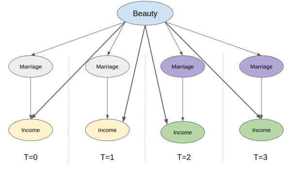
The trick is to see that, by zooming in a unit and tracking how it evolves over time, we are already controlling for anything that is fixed over time. That includes any time fixed unmeasured confounders. In the graph above, for instance, we can already know that the increase in income over time cannot be due to an increase in beauty, simply because beauty stays the same (it is time fixed after all). The bottom line is that even though we cannot control for beauty, since we can’t measure it, we can still use the panel structure so it is not a problem anymore.
Another way of seeing this is to think about these time fixed confounders as attributes that are specific to each unit. This would be equivalent to adding an intermediary unit node to our causal graph. Now, notice how controlling for the unit itself already blocks the backdoor path between the outcome and any of the unobserved but time fixed confounders.
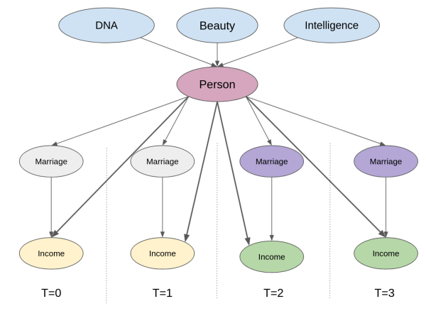
Think about it. We can’t measure attributes like beauty and intelligence, but we know that the person who has them is the same individual across time. The mechanics of actually doing this control is very simple. All we need to do is create dummy variables indicating that person and add that to a linear model. This is what we mean when we say we can control for the person itself: we are adding a variable (dummy in this case) that denotes that particular person. When estimating the effect of marriage on income with this person dummy in our model, regression finds the effect of marriage while keeping the person variable fixed. Adding this unit dummy is what we call a fixed effect model.
Fixed Effects#
To make matters more formal, let’s first take a look at the data that we have. Following our example, we will try to estimate the effect of marriage on income. Our data contains those 2 variables, married and lwage, on multiple individuals (nr) for multiple years. Notice that wage is in log form. In addition to this, we have other controls, like number of hours worked that year, years of education and so on.
data = wage_panel.load()
data.head()
| nr | year | black | ... | lwage | expersq | occupation | |
|---|---|---|---|---|---|---|---|
| 0 | 13 | 1980 | 0 | ... | 1.197540 | 1 | 9 |
| 1 | 13 | 1981 | 0 | ... | 1.853060 | 4 | 9 |
| 2 | 13 | 1982 | 0 | ... | 1.344462 | 9 | 9 |
| 3 | 13 | 1983 | 0 | ... | 1.433213 | 16 | 9 |
| 4 | 13 | 1984 | 0 | ... | 1.568125 | 25 | 5 |
5 rows × 12 columns
Generally, the fixed effect model is defined as
\( y_{it} = \beta X_{it} + \gamma U_i + e_{it} \)
where \(y_{it}\) is the outcome of individual \(i\) at time \(t\), \(X_{it}\) is the vector of variables for individual \(i\) at time \(t\). \(U_i\) is a set of unobservables for individual \(i\). Notice that those unobservables are unchanging through time, hence the lack of the time subscript. Finally, \(e_{it}\) is the error term. For the education example, \(y_{it}\) is log wages, \(X_{it}\) are the observable variables that change in time, like marriage and experience and \(U_i\) are the variables that are not observed but constant for each individual, like beauty and intelligence.
Now, remember how I’ve said that using panel data with a fixed effect model is as simple as adding a dummy for the entities. It’s true, but in practice, we don’t actually do it. Imagine a dataset where we have 1 million customers. If we add one dummy for each of them, we would end up with 1 million columns, which is probably not a good idea. Instead, we use the trick of partitioning the linear regression into 2 separate models. We’ve seen this before, but now is a good time to recap it. Suppose you have a linear regression model with a set of features \(X_1\) and another set of features \(X_2\).
\( \hat{Y} = \hat{\beta_1} X_1 + \hat{\beta_2} X_2 \)
where \(X_1\) and \(X_2\) are feature matrices (one row per feature and one column per observation) and \(\hat{\beta_1}\) and \(\hat{\beta_2}\) are row vectors. You can get the exact same \(\hat{\beta_1}\) parameter by doing
regress the outcome \(y\) on the second set of features \(\hat{y^*} = \hat{\gamma_1} X_2\)
regress the first set of features on the second \(\hat{X_1} = \hat{\gamma_2} X_2\)
obtain the residuals \(\tilde{X}_1 = X_1 - \hat{X_1}\) and \(\tilde{y}_1 = y_1 - \hat{y^*}\)
regress the residuals of the outcome on the residuals of the features \(\hat{y} = \hat{\beta_1} \tilde{X}_1\)
The parameter from this last regression will be exactly the same as running the regression with all the features. But how exactly does this help us? Well, we can break the estimation of the model with the entity dummies into 2. First, we use the dummies to predict the outcome and the feature. These are steps 1 and 2 above.
Now, remember how running a regression on a dummy variable is as simple as estimating the mean for that dummy? If you don’t, let’s use our data to show how this is true. Let’s run a model where we predict wages as a function of the year dummy.
mod = smf.ols("lwage ~ C(year)", data=data).fit()
mod.summary().tables[1]
| coef | std err | t | P>|t| | [0.025 | 0.975] | |
|---|---|---|---|---|---|---|
| Intercept | 1.3935 | 0.022 | 63.462 | 0.000 | 1.350 | 1.437 |
| C(year)[T.1981] | 0.1194 | 0.031 | 3.845 | 0.000 | 0.059 | 0.180 |
| C(year)[T.1982] | 0.1782 | 0.031 | 5.738 | 0.000 | 0.117 | 0.239 |
| C(year)[T.1983] | 0.2258 | 0.031 | 7.271 | 0.000 | 0.165 | 0.287 |
| C(year)[T.1984] | 0.2968 | 0.031 | 9.558 | 0.000 | 0.236 | 0.358 |
| C(year)[T.1985] | 0.3459 | 0.031 | 11.140 | 0.000 | 0.285 | 0.407 |
| C(year)[T.1986] | 0.4062 | 0.031 | 13.082 | 0.000 | 0.345 | 0.467 |
| C(year)[T.1987] | 0.4730 | 0.031 | 15.232 | 0.000 | 0.412 | 0.534 |
Notice how this model is predicting the average income in 1980 to be 1.3935, in 1981 to be 1.5129 (1.3935+0.1194) and so on. Now, if we compute the average by year, we get the exact same result. (Remember that the base year, 1980, is the intercept. So you have to add the intercept to the parameters of the other years to get the mean lwage for the year).
data.groupby("year")["lwage"].mean()
year
1980    1.393477
1981    1.512867
1982    1.571667
1983    1.619263
1984    1.690295
1985    1.739410
1986    1.799719
1987    1.866479
Name: lwage, dtype: float64
This means that if we get the average for every person in our panel, we are essentially regressing the individual dummy on the other variables. This motivates the following estimation procedure:
Create time-demeaned variables by subtracting the mean for the individual:
\(\ddot{Y}_{it} = Y_{it} - \bar{Y}_i\)
\(\ddot{X}_{it} = X_{it} - \bar{X}_i\)Regress \(\ddot{Y}_{it}\) on \(\ddot{X}_{it}\)
Notice that when we do so, the unobserved \(U_i\) vanishes. Since \(U_i\) is constant across time, we have that \(\bar{U_i}=U_i\). If we have the following system of two equations
And we subtract one from the other, we get
which wipes out all unobserved that are constant across time. To be honest, not only do the unobserved variables vanish. This happens to all the variables that are constant in time. For this reason, you can’t include any variables that are constant across time, as they would be a linear combination of the dummy variables and the model wouldn’t run.

To check which variables are those, we can group our data by individual and get the sum of the standard deviations. If it is zero, it means the variable isn’t changing across time for any of the individuals.
data.groupby("nr").std().sum()
year            1334.971910
black              0.000000
exper           1334.971910
hisp               0.000000
hours         203098.215649
married          140.372801
educ               0.000000
union            106.512445
lwage            173.929670
expersq        17608.242825
occupation       739.222281
dtype: float64
For our data, we need to remove ethnicity dummies, black and hisp, since they are constant for the individual. Also, we need to remove education. We will also not use occupation, since this is probably mediating the effect of marriage on wage (it could be that single men are able to take more time demanding positions). Having selected the features we will use, it’s time to estimate this model.
To run our fixed effect model, first, let’s get our mean data. We can achieve this by grouping everything by individuals and taking the mean.
Y = "lwage"
T = "married"
X = [T, "expersq", "union", "hours"]

mean_data = data.groupby("nr")[X+[Y]].mean()
mean_data.head()
| married | expersq | union | hours | lwage | |
|---|---|---|---|---|---|
| nr | |||||
| 13 | 0.000 | 25.5 | 0.125 | 2807.625 | 1.255652 |
| 17 | 0.000 | 61.5 | 0.000 | 2504.125 | 1.637786 |
| 18 | 1.000 | 61.5 | 0.000 | 2350.500 | 2.034387 |
| 45 | 0.125 | 35.5 | 0.250 | 2225.875 | 1.773664 |
| 110 | 0.500 | 77.5 | 0.125 | 2108.000 | 2.055129 |
To demean the data, we need to set the index of the original data to be the individual identifier, nr. Then, we can simply subtract one data frame from the mean data frame.
demeaned_data = (data
               .set_index("nr") # set the index as the person indicator
               [X+[Y]]
               - mean_data) # subtract the mean data

demeaned_data.head()
| married | expersq | union | hours | lwage | |
|---|---|---|---|---|---|
| nr | |||||
| 13 | 0.0 | -24.5 | -0.125 | -135.625 | -0.058112 |
| 13 | 0.0 | -21.5 | 0.875 | -487.625 | 0.597408 |
| 13 | 0.0 | -16.5 | -0.125 | 132.375 | 0.088810 |
| 13 | 0.0 | -9.5 | -0.125 | 152.375 | 0.177561 |
| 13 | 0.0 | -0.5 | -0.125 | 263.375 | 0.312473 |
Finally, we can run our fixed effect model on the time-demeaned data.
mod = smf.ols(f"{Y} ~ {'+'.join(X)}", data=demeaned_data).fit()
mod.summary().tables[1]
| coef | std err | t | P>|t| | [0.025 | 0.975] | |
|---|---|---|---|---|---|---|
| Intercept | -6.679e-17 | 0.005 | -1.32e-14 | 1.000 | -0.010 | 0.010 |
| married | 0.1147 | 0.017 | 6.756 | 0.000 | 0.081 | 0.148 |
| expersq | 0.0040 | 0.000 | 21.958 | 0.000 | 0.004 | 0.004 |
| union | 0.0784 | 0.018 | 4.261 | 0.000 | 0.042 | 0.115 |
| hours | -8.46e-05 | 1.25e-05 | -6.744 | 0.000 | -0.000 | -6e-05 |
If we believe that fixed effect eliminates the all omitted variable bias, this model is telling us that marriage increases a man’s wage by 11%. This result is very significant. One detail here is that for fixed effect models, the standard errors need to be clustered. So, instead of doing all our estimation by hand (which is only nice for pedagogical reasons), we can use the library linearmodels and set the argument cluster_entity to True.
from linearmodels.panel import PanelOLS
mod = PanelOLS.from_formula("lwage ~ expersq+union+married+hours+EntityEffects",
                            data=data.set_index(["nr", "year"]))

result = mod.fit(cov_type='clustered', cluster_entity=True)
result.summary.tables[1]
| Parameter | Std. Err. | T-stat | P-value | Lower CI | Upper CI | |
|---|---|---|---|---|---|---|
| expersq | 0.0040 | 0.0002 | 16.552 | 0.0000 | 0.0035 | 0.0044 |
| union | 0.0784 | 0.0236 | 3.3225 | 0.0009 | 0.0322 | 0.1247 |
| married | 0.1147 | 0.0220 | 5.2213 | 0.0000 | 0.0716 | 0.1577 |
| hours | -8.46e-05 | 2.22e-05 | -3.8105 | 0.0001 | -0.0001 | -4.107e-05 |
Notice how the parameter estimates are identical to the ones we’ve got with time-demeaned data. The only difference is that the standard errors are a bit larger. Now, compare this to the simple OLS model that doesn’t take the time structure of the data into account. For this model, we add back the variables that are constant in time.
mod = smf.ols("lwage ~ expersq+union+married+hours+black+hisp+educ", data=data).fit()
mod.summary().tables[1]
| coef | std err | t | P>|t| | [0.025 | 0.975] | |
|---|---|---|---|---|---|---|
| Intercept | 0.2654 | 0.065 | 4.103 | 0.000 | 0.139 | 0.392 |
| expersq | 0.0032 | 0.000 | 15.750 | 0.000 | 0.003 | 0.004 |
| union | 0.1829 | 0.017 | 10.598 | 0.000 | 0.149 | 0.217 |
| married | 0.1410 | 0.016 | 8.931 | 0.000 | 0.110 | 0.172 |
| hours | -5.32e-05 | 1.34e-05 | -3.978 | 0.000 | -7.94e-05 | -2.7e-05 |
| black | -0.1347 | 0.024 | -5.679 | 0.000 | -0.181 | -0.088 |
| hisp | 0.0132 | 0.021 | 0.632 | 0.528 | -0.028 | 0.054 |
| educ | 0.1057 | 0.005 | 22.550 | 0.000 | 0.097 | 0.115 |
This model is saying that marriage increases the man’s wage by 14%. A somewhat larger effect than the one we found with the fixed effect model. This suggests some omitted variable bias due to fixed individual factors, like intelligence and beauty, not being added to the model.
Visualizing Fixed Effects#
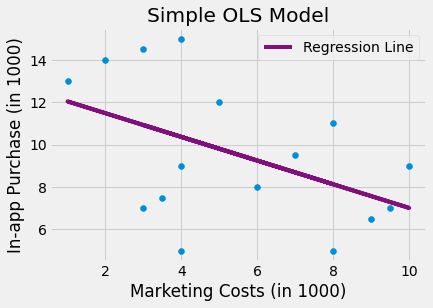
To expand our intuition about how fixed effect models work, let’s diverge a little to another example. Suppose you work for a big tech company and you want to estimate the impact of a billboard marketing campaign on in-app purchase. When you look at data from the past, you see that the marketing department tends to spend more to place billboards on cities where the purchase level is lower. This makes sense right? They wouldn’t need to do lots of advertisement if sales were skyrocketing. If you run a regression model on this data, it looks like higher cost in marketing leads to less in-app purchase, but only because marketing investments is biased towards low spending regions.
Knowing a lot about causal inference, you decide to run a fixed effect model, adding the city’s indicator as a dummy variable to your model. The fixed effect model controls for city specific characteristics that are constant in time, so if a city is less open to your product, it will capture that. When you run that model, you can finally see that more marketing costs leads to higher in-app purchase.
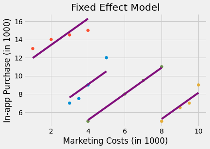
Take a minute to appreciate what the image above is telling you about what fixed effect is doing. Notice that fixed effect is fitting one regression line per city. Also notice that the lines are parallel. The slope of the line is the effect of marketing costs on in-app purchase. So the fixed effect is assuming that the causal effect is constant across all entities, which are cities in this case. This can be a weakness or an advantage, depending on how you see it. It is a weakness if you are interested in finding the causal effect per city. Since the FE model assumes this effect is constant across entities, you won’t find any difference in the causal effect. However, if you want to find the overall impact of marketing on in-app purchase, the panel structure of the data is a very useful leverage that fixed effects can explore.
Time Effects#
Just like we did a fixed effect for the individual level, we could design a fixed effect for the time level. If adding a dummy for each individual controls for fixed individual characteristics, adding a time dummy would control for variables that are fixed for each time period, but that might change across time. One example of such a variable is inflation. Prices and salary tend to go up with time, but the inflation on each time period is the same for all entities. To give a more concrete example, suppose that marriage is increasing with time. If the wage and marriage proportion also changes with time, we would have time as a confounder. Since inflation also makes salary increase with time, some of the positive association we see between marriage and wage would be simply because both are increasing with time. To correct for that, we can add a dummy variable for each time period. In linear models, this is as simple as adding TimeEffects to our formula and setting the cluster_time to true.
mod = PanelOLS.from_formula("lwage ~ expersq+union+married+hours+EntityEffects+TimeEffects",
                            data=data.set_index(["nr", "year"]))

result = mod.fit(cov_type='clustered', cluster_entity=True, cluster_time=True)
result.summary.tables[1]
| Parameter | Std. Err. | T-stat | P-value | Lower CI | Upper CI | |
|---|---|---|---|---|---|---|
| expersq | -0.0062 | 0.0008 | -8.1479 | 0.0000 | -0.0077 | -0.0047 |
| union | 0.0727 | 0.0228 | 3.1858 | 0.0015 | 0.0279 | 0.1174 |
| married | 0.0476 | 0.0177 | 2.6906 | 0.0072 | 0.0129 | 0.0823 |
| hours | -0.0001 | 3.546e-05 | -3.8258 | 0.0001 | -0.0002 | -6.614e-05 |
In this new model, the effect of marriage on wage decreased significantly from 0.1147 to 0.0476. Still, this result is significant at a 99% level, so man could still expect an increase in earnings from marriage.
When Panel Data Won’t Help You#
Using panel data and fixed effects models is an extremely powerful tool for causal inference. When you don’t have random data nor good instruments, the fixed effect is as convincing as it gets for causal inference with non experimental data. Still, it is worth mentioning that it is not a panacea. There are situations where even panel data won’t help you.
The most obvious one is when you have confounders that are changing in time. Fixed effects can only eliminate bias from attributes that are constant for each individual. For instance, suppose that you can increase your intelligence level by reading books and eating lots of good fats. This causes you to get a higher paying job and a wife. Fixed effect won’t be able to remove this bias due to unmeasured intelligence confounding because, in this example, intelligence is changing in time.

Another less obvious case when fixed effect fails is when you have reversed causality. For instance, let’s say that it isn’t marriage that causes you to earn more. Is earning more that increases your chances of getting married. In this case, it will appear that they have a positive correlation but earnings come first. They would change in time and in the same direction, so fixed effects wouldn’t be able to control for that.
Key Ideas#
Here, we saw how to use panel data, data where we have multiple measurements of the same individuals across multiple time periods. When that is the case, we can use a fixed effect model that controls for the entity, holding all individual, time constant attributes, fixed. This is a powerful and very convincing way of controlling for confounding and it is as good as it gets with non random data.
Finally, we saw that FE is not a panacea. We saw two situations where it doesn’t work: when we have reverse causality and when the unmeasured confounding is changing in time.
References#
I like to think of this entire book as a tribute to Joshua Angrist, Alberto Abadie and Christopher Walters for their amazing Econometrics class. Most of the ideas here are taken from their classes at the American Economic Association. Watching them is what is keeping me sane during this tough year of 2020.
I’ll also like to reference the amazing books from Angrist. They have shown me that Econometrics, or ‘Metrics as they call it, is not only extremely useful but also profoundly fun.
Another important reference is Miguel Hernan and Jamie Robins’ book. It has been my trustworthy companion in the most thorny causal questions I had to answer.
Finally, I’d also like to compliment Scott Cunningham and his brilliant work mingling Causal Inference and Rap quotes:

Contribute#
Causal Inference for the Brave and True is an open-source material on causal inference, the statistics of science. It uses only free software, based in Python. Its goal is to be accessible monetarily and intellectually. If you found this book valuable and you want to support it, please go to Patreon. If you are not ready to contribute financially, you can also help by fixing typos, suggesting edits or giving feedback on passages you didn’t understand. Just go to the book’s repository and open an issue. Finally, if you liked this content, please share it with others who might find it useful and give it a star on GitHub.